Anomaly Detection Using H2O Deep Learning
Hortonworks DataFlow is an integrated platform that makes data ingestion fast, easy, and secure. Download the white paper now. Brought to you in partnership with Hortonworks.
In a previous article, we had an overview of the applications of Deep Learning and touched upon some basic points to consider while creating a Deep Learning model. We also had an overview of what it is and methods to get started with deep learning. In this article, we jump straight into creating an anomaly detection model using Deep Learning and anomaly package from H2O.
Anomaly Detection
Readers who don't know what it is can view it as anything that occurs unexpected and is a rare event. It is a deviation from the standard pattern and does not confirm to the usual behavior of the data. Let's say we work in a steel manufacturing industry, and we see the quality of the steel suddenly drops down below the permissible limits. This is an anomaly; if not detected and resolved soon will cost the organization millions. So to detect an anomaly at an early stage of its occurrence is very crucial.
There are various methods for anomaly detection which can be either rule-based or machine-learning-based detection systems. Rule-based systems are usually designed by defining rules that describe an anomaly and assigning thresholds and limits. For example, anything above the threshold or below is classified as an anomaly. Rule-based systems are designed from the experience of the industry experts and can be thought of as systems that are designed to detect “known anomalies”. They are "known anomalies" because we recognize what is usual and what is not usual.
However, if there is something that is not known and has never been discovered so far, then creating rules for detecting anomalies is difficult. In such cases, machine learning-based detection systems come in handy. They are a bit complicated but can deal with many uncertain situations. Mostly, they can deduce the patterns that are unusual and alert the users. The one technique we demonstrate here is using H2O's autoencoder deep learning with anomaly package.
For some more techniques for anomaly detection such as one class SVM, you can refer my upcoming book on Data Science using Oracle Data Miner and Oracle R Enterprise published by Apress (Aforementioned is a short excerpt from my book).
The Dataset Used for This Demo
The data was extracted from the 1974 Motor Trend US magazine and comprises fuel consumption and ten aspects of automobile design and performance for 32 automobiles (1973–74 models). The Data Set was modified a bit to introduce some data anomalies.The data set and code for this demonstration were prepared for the meetup Data Science for IoT using H2O, London by me, Ajit Jaokar and Jo-Fai Chow from H2O.ai who had guided me on H2O stuff. However, I missed attending the D-Day.
We can install and get started using H2O in R using the below script.
Note: We are using H2O with R for the demo. However, the beauty of H2O is that you can kick it up for your machine learning tasks using any of the popular languages - Python and Java.
So, let's get started with detecting the anomalies and separate the unknowns from the knowns.
Installation
If you have an older version of H2O installed, this script will remove it and install the latest one.
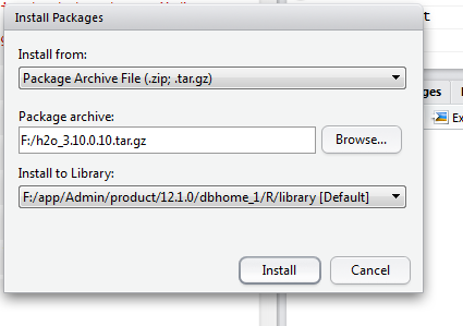
If you find difficulty in installing H2O using the above script, then download the tar file from http://h2o-release.s3.amazonaws.com/h2o/rel-turing/10/R/src/contrib/h2o_3.10.0.10.tar.gz Install it by loading the downloaded package archive from tools -> install package as shown in below figure.
If you already have H2O installed, then we can skip running the above script and load the H2O libraries as shown in the below figure. The code h20.init() start the h2o server. It provides the method to specify the number of threads, IP and Port to be used by H20. By default, H2O is limited to the CRAN default of 2 CPUs. If you have more than 2 CPU, you can use all of those by passing the parameter nthreads=-1 to the h2o.init function.
After starting H2O, you can use and view every operation done over H2O in the Web UI at http://localhost:54321
Reading the Data
Next, we read the data into the mtcar variables and change the datatype of some variables to factors as shown below. We convert them into factors as there have few distinct values and so treating them as categories will help for better analysis.
Alternatively, we can use h2o.importFile and h2o.uploadFile to read files. You can use h2o.uploadFile to upload a file from your local disk. It is a push from the client to the server and is only intended for smaller data sizes. h2o.importFile is another function which pulls information from the server from a location specified by the client. It is more suitable for big-data operations. Using h2o.importFile, you can also import files stored in HDFS as well as load an entire folder of files.
You can also use as.h2o() to import a local R data frame to the H2O. It serially uploads the file to H2O and so might be a bit slower than other file import methods.
Training an Autoencoder
An autoencoder neural network is a class of Deep Learning that can be used for unsupervised learning. Anomaly detection depends essentially on unsupervised techniques as we tend to find unknown from the knowns. So, we can say the data set for anomaly detection has just one class i.e. "known" and is not suitable for supervised learning. The autoencoder algorithm applies backpropagation, setting the target values to be equal to the inputs.
We can use the h2o.deeplearning library setting autoencoder= TRUE to train our autoencoder model.
To go through the complete list of parameters, one can refer r_h20_deep_learning reference page. Also, there is a great tutorial on Deep Learning using H2O by Erin LeDell, Data Scientist, H2O.ai

The h2o.anomaly function can be used to detect anomalies in a dataset. This function uses an H2O autoencoder model. This function reconstructs the original data set using the model and calculates the Mean Squared Error(MSE) for each data point.
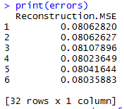
Next, we plot the reconstruction.MSE and see where the model grapples to reconstruct the original records. This means that the model was not able to learn patterns for those records correctly which can be an anomaly.
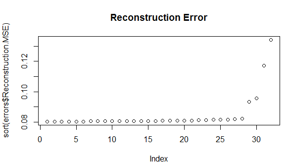
It is normal for a good generalized model to show some variations in reconstruction. So, every little variation in reconstruction cannot be considered as an anomaly. We define a cutoff point to hold only records above reconstruction error as 0.099 as an anomaly.
P.C: https://dzone.com/articles/dive-deep-into-deep-learning-using-h2o-1?utm_medium=feed&utm_source=feedpress.me&utm_campaign=Feed:%20dzone


Post a Comment